GAM-ZOTS Toolbox Manual
Last News:
Version GAM-ZOTS_toolbox_v1.1 is available. A GUI (Graphical User Interface) option to run the GAM-ZOTS Toolbox was been developed. September 30, 2019.
This toolbox contains the proposed learning approach to design a neo-fuzzy neuron for identification purposes using backfitting algorithm published in:
Jérôme Mendes, Francisco Souza, Rui Araújo, and Saeid Rastegar. Neo-fuzzy neuron learning using backfitting algorithm. Neural Computing and Applications, 31(8):3609–3618, August 2019. [doi].
Abstract: An automatic and simple approach to design a neo-fuzzy neuron for identification purposes is proposed. The proposed approach uses the backfitting algorithm to learn multiple univariate additive models, where each additive model is a zero-order T-S fuzzy system which is a function of one input variable, and there is one additive model for each input variable. The multiple zero-order T-S fuzzy models constitute a neo-fuzzy neuron. The structure of the model used in this paper allows to have results with good interpretability and accuracy.
Software source code: GAM-ZOTS Toolbox (Matlab implementation)
How to Run
For use with Matlab. You can run the GAM-ZOTS toolbox with GUI (Graphical User Interface), Main.m, or without, Main_noGUI.m.
Main_noGUI.m – Just run the Main_noGUI.m file to start GAM-ZOTS toolbox without a GUI.
Main.m – Run the Main.m file, and a GUI will appear (Figure 1) to configure the main parameters. Click in “Run”.
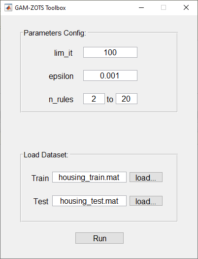
Figure 1: Initial GUI interface of GAM-ZOTS toolbox.
Main Functions
Main.m – This is the main function to run GAM-ZOTS toolbox with a GUI.
Main_noGUI.m – This is the main function to run GAM-ZOTS toolbox without a GUI.
C_BestNumberRules.m - This function returns the best number of rules from the candidate ones.
C_FAM.m - This function represents the learning algorithm (Algorithm 2).
Initialization.m - This function initializes the struct x, i.e. the initial parameters (Algorithm 2 Step 2).
AdditiveModels_C.cpp – This mex function is responsible to the Consequent Design, Algorithm 2 Step 3.
FinalyModel_C.cpp - This mex function gives the estimation of the learned neo-fuzzy neuro system.
PlotMFs.m - This function presents the plots of the membership functions of all input variables.
Main Configuration Files
ParametersConfig_noGUI.m – This file contains the main variables of the algorithm:
\(lim_{it}\) - Maximal number of learning interactions.
\(\epsilon\)- Termination condition defined on Algorithm 2 Step 3.c.ii.
Number of rules per input variable - The learning algorithm will run varying the fuzzy rules as defined by the user. On the paper as from 2 to 20 rules.
DatasetConfig_noGUI.m – This file contains the definition of the dataset. Change it to test on another dataset.
Configuration on the GUI interface: Using the Graphical User Interface (GUI), the above parameters presented on ParametersConfig_noGUI.m and DatasetConfig_manually.m are defined on the GUI (see Figure 1).
Definition of the Struct x
x is a struct, in which, contains all parameters of the neo-fuzzy neuron system.
Elements of struct x, Rows: contain all parameters of the zero-order T-S fuzzy system for each input variable, e.g.:
row 1 contains the parameters of the zero-order T-S fuzzy system for the input variable \(x_1\)
row j contains the parameters of the zero-order T-S fuzzy system for the input variable \(x_j\)
Figure 2 contains the parameters of the 13 input variables of the Boston Housing dataset.
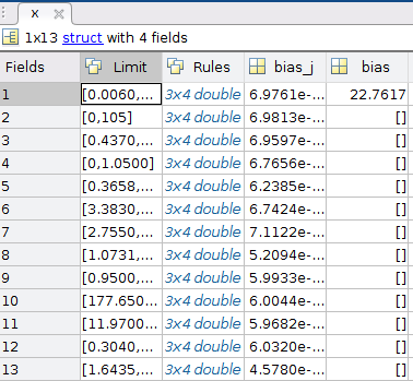
Figure 2: Example of struct x. Final values of the current example, Boston Housing dataset.
Elements of struct x, Columns:
First column: contains the limits of the universe of discourse of the respective input variable.
Second column: contain the matrix rules of the respective input variable (Figure 3):
Rows: each row represents a fuzzy rule;
1º column: represents parameter \(a_{j,i}\) (lower limit of the respective membership function);
2º column: represents parameter \(b_{j,i}\) (center value of the respective membership function);
3º column: represents parameter \(c_{j,i}\) (upper limit of the respective membership function);
4º column: represents the consequent parameter of the respective rule, \(\theta_{j,i}\).
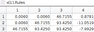
Figure 3: Example of the matrix rules.
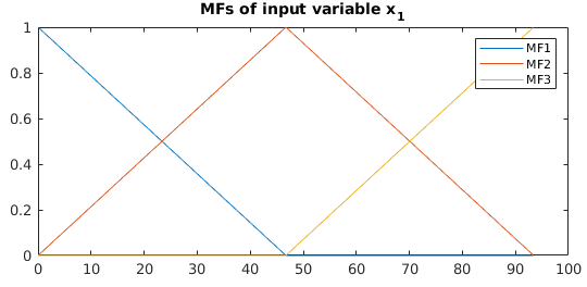
Figure 4: Plot of MFs represented on Figure 3.
Third column: represents the bias (\(bias_j\)) of the model of the respective input variable,
Fourth column: represents the bias (\(y_0\)) of the general model. Just the first row is used.
A Simple Script
The main example (file Main.m) runs in order to find the best number of rules from the candidate ones, like the paper, in which, the learning algorithm is tested by varying the number of fuzzy rules between 2 and 20. This script is much faster since not use cross-validation to find the best number of rules. In the script Simple_script.m , the number of rules is defined by the user, and it is unique (scalar, not a vector of possible candidates).
You can run the simple script with a GUI Simple_script.m (Figure 5), or without, Simple_script_noGUI.m.
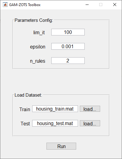
Figure 5: Initial GUI interface of Simple_Script of GAM-ZOTS toolbox.
Results presented in the GUI
Using the GUI to run the GAM-ZOTS toolbox the results are presented on the GUI represented by Figure 6, in which,
it can be seen the training and testing errors;
it can plot the final membership function of all input variables or on just a specific input variable;
and it can plot the estimated output variable on the train and test datasets.
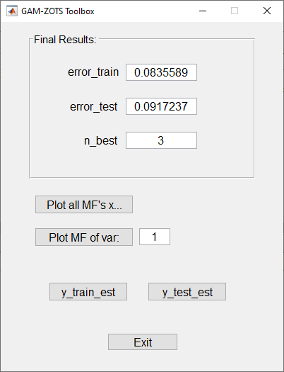
Figure 6: Results GUI interface of GAM-ZOTS toolbox.